Monte Carlo Simulation in Python

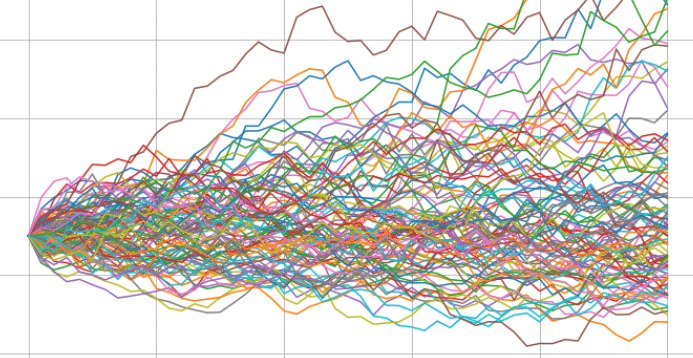
Today, we will explore the concept of Monte Carlo simulation and how it can be implemented using Python. Monte Carlo simulation is a computational technique that uses random sampling to model and analyse complex systems. It is widely used in various fields such as finance, physics and engineering for solving problems that are difficult or impossible to solve analytically.

Prerequisites

Before we begin, make sure you have the following installed:

• Python (version 3.x)
• Jupyter Notebook or any Python IDE of your choice

What is Monte Carlo Simulation?

Monte Carlo simulation is a statistical technique that allows us to estimate the probability of certain outcomes by running multiple random trials. It is based on the law of large numbers, which states that as the number of trials increases, the average of the observed values will converge to the expected value.

The basic steps involved in a Monte Carlo simulation are as follows:

1. Define the problem: Clearly define the problem and the variables involved.
2. Generate random inputs: Generate random values for the variables based on their probability distributions.
3. Perform calculations: Use the generated inputs to perform the necessary calculations.
4. Repeat steps 2 and 3: Repeat steps 2 and 3 a large number of times to get a statistically significant result.
5. Analyse the results: Analyse the results to draw conclusions and make decisions.

Example 1: Estimating Pi using Monte Carlo Simulation

Let's start with a simple example to estimate the value of Pi using Monte Carlo simulation. The idea is to randomly generate points within a square and see how many of them fall within a quarter of a circle inscribed in the square.

Step 1: Define the problem

We want to estimate the value of Pi using Monte Carlo simulation.

Step 2: Generate random inputs

We need to generate random points within a square. We can do this by generating random x and y coordinates between -1 and 1.

import random

def generate_random_point():
    x = random.uniform(-1, 1)
    y = random.uniform(-1, 1)
    return x, y

Step 3: Perform calculations

We need to check if the generated points fall within the quarter of a circle inscribed in the square. We can do this by calculating the distance of each point from the origin and checking if it is less than or equal to 1.

def is_point_inside_circle(x, y):
    distance = (x ** 2 + y ** 2) ** 0.5
    return distance <= 1

Step 4: Repeat steps 2 and 3

We will repeat steps 2 and 3 a large number of times to get a statistically significant result. Let's say we want to generate 1 million random points.

num_points = 1000000
num_points_inside_circle = 0

for _ in range(num_points):
    x, y = generate_random_point()
    if is_point_inside_circle(x, y):
        num_points_inside_circle += 1

Step 5: Analyse the results

Finally, we can estimate the value of Pi using the formula:

pi_estimate = 4 * (num_points_inside_circle / num_points)
print("Estimated value of Pi:", pi_estimate)

Example 2: Estimating Stock Portfolio Value

In this example, we will estimate the value of a stock portfolio after a given time period. We will assume that the daily returns of each stock in the portfolio follow a normal distribution.

Step 1: Define the problem

We want to estimate the value of a stock portfolio after a given time period using Monte Carlo simulation.

Step 2: Generate random inputs

We need to generate random daily returns for each stock in the portfolio. We can do this by sampling from a normal distribution with the mean and standard deviation of the historical returns of each stock.

import numpy as np

# Historical returns of each stock in the portfolio
stock_returns = [0.05, 0.03, 0.02, 0.04]

def generate_daily_returns():
    return np.random.normal(stock_returns, 0.01, len(stock_returns))

Step 3: Perform calculations

We need to calculate the cumulative returns of the portfolio over the given time period. We can do this by multiplying the daily returns with the initial portfolio value.

initial_portfolio_value = 100000

def calculate_portfolio_value(daily_returns):
    portfolio_value = initial_portfolio_value
    for daily_return in daily_returns:
        portfolio_value *= (1 + daily_return)
    return portfolio_value

Step 4: Repeat steps 2 and 3

We will repeat steps 2 and 3 a large number of times to get a distribution of possible portfolio values. Let's say we want to run 1000 simulations.

num_simulations = 1000
portfolio_values = []

for _ in range(num_simulations):
    daily_returns = generate_daily_returns()
    portfolio_value = calculate_portfolio_value(daily_returns)
    portfolio_values.append(portfolio_value)

Step 5: Analyse the results

We can analyse the distribution of portfolio values to estimate the expected value and the risk associated with the portfolio.

mean_portfolio_value = np.mean(portfolio_values)
std_portfolio_value = np.std(portfolio_values)

print("Expected portfolio value:", mean_portfolio_value)
print("Standard deviation of portfolio value:", std_portfolio_value)

Example 3: Pricing a European Option

In this example, we will use Monte Carlo simulation to price a European option. We will assume that the underlying asset follows a geometric Brownian motion.

Step 1: Define the problem

We want to price a European option using Monte Carlo simulation.

Step 2: Generate random inputs

We need to generate random stock prices at the option's expiration date. We can do this by simulating the stock price using the geometric Brownian motion equation.

initial_stock_price = 100
risk_free_rate = 0.05
volatility = 0.2
time_to_expiration = 1

def generate_stock_price():
    drift = (risk_free_rate - 0.5 * volatility ** 2) * time_to_expiration
    diffusion = volatility * np.sqrt(time_to_expiration) * np.random.normal()
    return initial_stock_price * np.exp(drift + diffusion)

Step 3: Perform calculations

We need to calculate the payoff of the option at the expiration date. For a European call option, the payoff is the maximum of zero and the difference between the stock price and the strike price.

strike_price = 110

def calculate_option_payoff(stock_price):
    return max(0, stock_price - strike_price)

Step 4: Repeat steps 2 and 3

We will repeat steps 2 and 3 a large number of times to get a distribution of possible option payoffs. Let's say we want to run 10000 simulations.

num_simulations = 10000
option_payoffs = []

for _ in range(num_simulations):
    stock_price = generate_stock_price()
    option_payoff = calculate_option_payoff(stock_price)
    option_payoffs.append(option_payoff)

Step 5: Analyse the results

We can analyse the distribution of option payoffs to estimate the expected value and the risk associated with the option.

mean_option_payoff = np.mean(option_payoffs)
std_option_payoff = np.std(option_payoffs)

print("Expected option payoff:", mean_option_payoff)
print("Standard deviation of option payoff:", std_option_payoff)

These are just two examples of Monte Carlo simulation applications. You can apply this technique to various other problems in different domains.

Final Example: Trajectory of a projectile

Monte Carlo simulation in Python that simulates the trajectory of a projectile under the influence of gravity:

import random
import math

def monte_carlo_simulation(num_simulations):
    num_hits = 0

    for _ in range(num_simulations):
        # Generate random initial velocity and angle
        initial_velocity = random.uniform(10, 30)
        angle = random.uniform(30, 60)

        # Convert angle to radians
        angle_rad = math.radians(angle)

        # Calculate initial horizontal and vertical velocities
        initial_vx = initial_velocity * math.cos(angle_rad)
        initial_vy = initial_velocity * math.sin(angle_rad)

        # Calculate time of flight
        time_of_flight = (2 * initial_vy) / 9.81

        # Calculate horizontal distance traveled
        horizontal_distance = initial_vx * time_of_flight

        # Check if the projectile hits the target
        if horizontal_distance >= 27:
            num_hits += 1

    # Calculate the probability of hitting the target
    probability = num_hits / num_simulations

    return probability

# Run the Monte Carlo simulation with 100,000 simulations
num_simulations = 100000
probability = monte_carlo_simulation(num_simulations)

print(f"Probability of hitting the target: {probability}")

In this example, the monte_carlo_simulation function takes the number of simulations as an input and performs the simulation. Inside the loop, random initial velocity and angle values are generated within specified ranges. The initial velocity is then split into horizontal and vertical components using trigonometry.

The time of flight is calculated using the vertical velocity and the acceleration due to gravity. The horizontal distance traveled is then calculated using the horizontal velocity and the time of flight.

If the horizontal distance is greater than or equal to 27 (indicating a hit on the target), the num_hits counter is incremented. Finally, the probability of hitting the target is calculated by dividing the number of hits by the total number of simulations.

The simulation is run with 100,000 simulations and the resulting probability is printed.